Linear algebra, i.e. the manipulation of vectors and matrices, has a fundamental role in computer graphics. The graphics pipeline is optimized to perform certain linear algebra computations in a single (vector) operation. In particular, seemingly different quantities, e.g. vertices, colors, textures, etc., can all be represented in a similar manner and manipulated using identical linear algebra operations. While a thorough understanding of linear algebra is not necessary to program computer graphics, a working knowledge is essential if one wishes to develop a new graphics API and/or write custom shaders that require user defined computations. This lab will introduce linear algebra in a 2D context, however these concepts will easily generalize to 3D (and even 4D) in the near future.
0. Getting Started
Download CS370_Lab03.zip, saving it into the labs directory.
Double-click on CS370_Lab03.zip and extract the contents of the archive into a subdirectory called CS370_Lab03
Navigate into the CS370_Lab03 directory and double-click on CS370_Lab03.sln (the file with the little Visual Studio icon with the 12 on it).
If the source file is not already open in the main window, open the source file by expanding the Source Files item in the Solution Explorer window and double-clicking transformHexagon.cpp.
1. Basic Linear Algebra Terminology
The fundamental concepts of linear algebra consist of vectors and matrices. We can think of a vector as a column of values (known as components of the vector). Hence a point in 2D space (x,y) would be represented by the vector

A matrix can be conceptualized as a table of values. Hence a 2x2 matrix (known as the dimension or size of the matrix where the first number represents the number of rows while the second number represents the number of columns) would be represented as
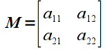
The elements of a matrix are typically indexed by row and column as shown above. Note that a vector is simply a special case of a matrix with a single column, i.e. an nx1 matrix. While technically a 1xn matrix, i.e. a single row, is often also referred to as a vector, we will reserve the term vector for a single column. Furthermore, matrices with the same number of rows as columns is known as a square matrix.
Vectors are typically represented programmatically as a 1D array while matrices are represented by a multi-dimensional array with corresponding element indexing.
2. Vector/Matrix Operations
Addition
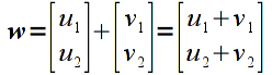
Addition is done componentwise for vectors/matricies that have the same dimensions. Hence adding two vectors
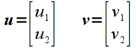
would give
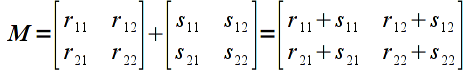
Similarly, adding matrices
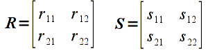
would give
However the computation
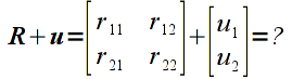
would be undefined since the two operands are of different sizes.
Multiplication
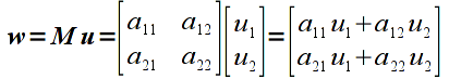
Multiplication is done for vectors/matrices that have matching inner dimensions, i.e. the number of columns of the first operand must be the same as the number of rows of the second operand. The resulting matrix will have a size corresponding to the outer dimensions, i.e. will have the same number of rows as the first operand and the same number of columns of the second operand. The elements of the resulting matrix are computed using the sum-of-products rule as shown below for a matrix multiplied by a vector (note a 2x2 matrix multiplied by a 2x1 vector results in a 2x1 vector, i.e. a vertex is transformed to a new vertex)
and a matrix multiplied by a matrix
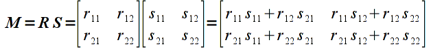
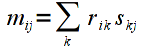
In general, for two matrices (including vectors) R ( m x k ) and S ( k x n ) the elements of the resulting product matrix M (of dimension m x n ) can be computed as
Note: Unlike regular arithmetic multiplication, matrix multiplication is not commutative, i.e. order is important. Hence if we multiply the same two matrices as above in the opposite order the result is
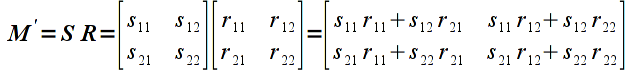
which in general will be different than the first product (there are certain special cases where they will be the same but we will assume that order matters). This property will become extremely important when we begin concatenating transformation matrices.
Tasks
For the six vertices from the last lab:

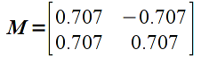
manually compute the new vertices that result from applying the following matrix transformation (i.e. perform matrix-vector multiplication for each vertex)
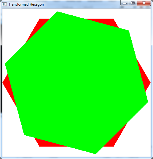
Add code to render_scene() to draw two polygons, one red using the original vertices and one green with the transformed ones. What is the difference between the two polygons?
Computing transformations by hand is cumbersome to say the least. I've included a function called Trans2D() that takes a transformation matrix as a 2D float array, a vector as a 1D float array, and an output vector as a 1D float array that will contain the transformed vector. Use this function along with the provided global variables to compute transformed vertices. Display the polygons with these two sets of vertices (note you can use the glVertex2fv() form to use an array as a vertex). Hint: Perform all the transformations before rendering the polygon with glBegin()/glEnd().
Experiment with different values of the matrix elements to see the resulting transformed polygons.
Compiling and running the program
Once you have completed typing in the code, you can build and run the program in one of two ways:
- Click the small green arrow in the middle of the top toolbar
- Hit F5 (or Ctrl-F5)
(On Linux/OSX: In a terminal window, navigate to the directory containing the source file and simply type make. To run the program type ./transformHexagon.exe)
The output should look similar to below
To quit the program simply close the window.
While we can always transform the vertices manually in our application, OpenGL provides various functions to apply transformations (MUCH more efficiently) within the graphics pipeline. Next time we will see how to take advantage of the capabilities provided by the graphics hardware to perform certain common transformations.
