Multi-texturing is a nice way to further enhance the appearance of surfaces in our scene without adding additional geometry. Unfortunately, the surface still appears flat, particularly with respect to lighting. One technique (that is based on multi-texturing) to create an even more realistic appearance of a rough surface is to adjust the normals to produce a self-shadowing effect known as bump mapping. Since normals are applied per vertex and then interpolated across the surface (per fragment) in the default pipeline, this would require using extremely complex geometries (similar to recursive subdivision) to capture sufficient surface detail. However we can simulate this effect through self-shadowing which gives the appearance of a slightly varying, i.e. rough, surface based on a normal map which is stored in a texture. This normal map (which being a texture is applied on a per pixel basis) can then be used in the fragment shader to define the varying normals per pixel in order to produce a changing lighting effect across each fragment, i.e. bump mapping. This will be done in addition to the application of a surface texture using the multi-texturing procedure from the last lab. However in order to perform the appropriate lighting calculation, we first need to transform the light vectors at each pixel into tangent space, i.e. such that the normal becomes the z-axis and two tangent vectors become the corresponding x and y axes. We then apply the modified normals according to the normal map texture and manually compute a new lighting color per pixel.

0. Getting Started

Download CS370_Lab22.zip, saving it into the labs directory.

Double-click on CS370_Lab22.zip and extract the contents of the archive into a subdirectory called CS370_Lab22

Navigate into the CS370_Lab22 directory and double-click on CS370_Lab22.sln (the file with the little Visual Studio icon with the 12 on it).

If the source file is not already open in the main window, open the source files by expanding the Source Files item in the Solution Explorer window and double-clicking bumpBall.cpp, bumpvert.vs, bumpfrag.fs, and sphere.h.

1. Tangent Space

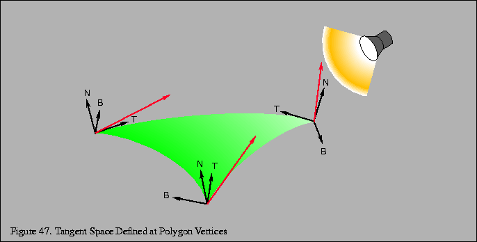
In order to apply bump mapping, we need to tranform the various lighting vectors into tangent space, i.e. the plane that is tangent to the surface with the vertex becoming the origin of the new coordinate system. This transformation makes the surface normal at the vertex the new z-axis (which simplifies the application of the bump map texture). Two additional perpendicular vectors, known as the tangent and binormal, will then define the tangent plane (i.e. become the x and y axes) - see the following figure.

Fortunately, we already have the normal (from the application) so we only need to define a tangent and then compute the vector cross product (see lab14) to give the binormal as:

The transformation matrix for the lighting vectors (assuming n, t, and b are unit vectors) is then given by

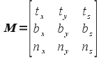
Multiplying this matrix by the corresponding light vectors (which transforms them to tangent space) can then easily be computed via three dot products with n, t, and b. The transformed light vectors can then be passed to the fragment shader to perform any desired per pixel lighting computation, e.g. the Phong model.

Tasks

• Add code to bumpvert.vs to define a global attribute vec3 variable named tangento. NOTE: This is an attribute variable since it will be set per vertex in the application.
• Add code to bumpvert.vs to define two global varying vec3 variables called lightv and viewv. These will be the transformed tangent space light vectors passed to the fragment shader.
• Add code to bumpvert.vs in main( ) to define a local vec3 variable named n and set it equal to the product of the normal matrix (i.e. gl_NormalMatrix) and the normal vector (i.e. gl_Normal). Normalize this vector using the built-in normalize( ) shader function. This will create the tangent space normal by applying any global transformations to the application defined normal.
• Add code to bumpvert.vs in main( ) to define a local vec3 variable named t and set it equal to the product of the normal matrix (i.e. gl_NormalMatrix) and the attribute vector tangento. Normalize this vector using the built-in normalize( ) shader function. This will create the tangent space tangent by applying any global transformations to the application defined tangent.
• Add code to bumpvert.vs in main( ) to define a local vec3 variable named b and set it equal to the cross product (using the built-in cross() shader function) of n and t. Since n and t are already unit vectors, the cross product will automatically also be a unit vector. This will create the tangent space binormal.
• Add code to bumpvert.vs in main( ) to define a local vec3 variable named viewe and set it equal to the vec3 product of the modelview matrix (i.e. gl_ModelViewMatrix) and the vertex vector (i.e. gl_Vertex). This will apply any global transformations to the application vertex to create the viewer vector.
• Add code to bumpvert.vs in main( ) to compute viewv.x as the dot product (using the built-in dot( ) shader function) between t and lighte. This will transform the first component of the light vector into tangent space.
• Add code to bumpvert.vs in main( ) to compute viewv.y as the dot product (using the built-in dot( ) shader function) between b and lighte. This will transform the second component of the light vector into tangent space.
• Add code to bumpvert.vs in main() to compute viewv.z as the dot product (using the built-in dot( ) shader function) between n and lighte. This will transform the third component of the light vector into tangent space.
• Add code to bumpvert.vs in main( ) to define a local vec3 variable named lighte and set it equal to the vec3 gl_LightSource[0].position minus viewe. Normalize this vector using the built-in normalize( ) shader function. This will create the light vector.
• Add code to bumpvert.vs in main( ) to compute the three components of lightv as the dot products (using the built-in dot( ) shader function) between t, b, and n similar to above. This will transform the light vector into tangent space.
• Add code to bumpvert.vs in main() to normalize lightv and viewv.

2. Normal Map Lighting

Once we have the light vectors (including the viewer vector) transformed to tangent space (which now has a normal given by (0,0,1)) for each fragment of the surface, we now wish to perturb the tangent space normal per pixel and compute a modified lighting effect to produce self-shadowing. To accomplish this effect, we will store the perturbed surface normals into a normal map which is essentially an "image" of the surface where the geometric variations are stored as colors (again utilizing the correspondence in the pipeline between 3D coordinates and RGB colors). This map is loaded into a texture and applied in addition to the surface texture using multi-texturing in the fragment shader. Since we are only slightly perturbing the direction of the normal, i.e. we primarily maintain the z-axis which is the blue channel, normal maps appear as a mainly blue image. Because we are unable to store negative values in color channels, we instead scale the values such that those between [0,0.5] represent negative values and those between [0.5,1] represent positive values. We can then obtain the original component values via the simple formula

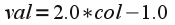
The new lighting components are then computed (via the Phong model) using the converted colors in the normal map and the transformed lighting vectors.

In particular, recall that the Phong diffuse factor is given by Lambert's law as

Tasks

• Add code in bumpfrag.fs to define two global varying vec3 variables named lightv and viewv. These are the tangent space light and viewer vectors computed in the vertex shader.
• Add code in bumpfrag.fs in main( ) to define a vec3 variable named Light and set it equal to a normalized lightv (since it may have been interpolated across the fragment during rasterization).
• Add code in bumpfrag.fs in main( ) to define a vec3 variable named normal and set it equal to a scaled version of bump.rgb (using the formula above) and normalize the result. This generates the new perturbed surface normal from the normal map color. (NOTE: This computation can be done in a single step as the operations will be performed component-wise.)
• Add code in bumpfrag.fs in main( ) to define a float variable named diffuse and set it equal to the maximum (using the built-in max() shader function) of the dot product between Light and normal and 0.0 (to clamp the resulting color).
• Add code to bumpfrag.fs in main( ) to compute gl_FragColor as the product of diffuse and texColor, i.e. blend the lighting color with the underlying texture.

3. Defining Tangent Vectors for Spheres

The final piece we need to do is define the tangent vector for our surface in the application and pass it to the vertex shader. Ideally we would like the tangent vector to point along what would be the s axis of the texture map when it is applied to the surface. If this is excessively cumbersome (or the normal map is sufficiently random), any vector perpendicular to the surface normal will work. Since the radius of a unit sphere is perpendicular to the surface, the normal vector at a point (x,y,z) is given in spherical coordinates as (which is identical to the original coordinates)

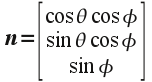
It is relatively straightforward to compute a perpendicular to this vector (see here for more details) as

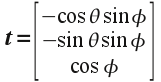
which can easily be verified via the dot product. We will assume that for the vertex (1,0,0) that the tangent is parallel to the z-axis giving the binormal as parallel to the y-axis. We will then rotate these vectors about the z-axis by an angle θ and then about the rotated y-axis by an angle φ (essentially obtaining the spherical coordinate transformation for the initial vertex). This procedure will provide well defined tangent vectors across the entire sphere.

In order to pass the tangent vector to the shaders, we first need to associate an attribute identifier (since it is per vertex) using the command

param = glGetAttribLocation(progObj, "var");

where param is a GLint that identifies the shader variable, progObj is the shader program object, and var is the name of the variable in the shader source we wish to associate (again enclosed in double quotes).

Whenever we wish to assign a value to the associated shader attribute variable (within a glBegin()/glEnd() construct) we simply call

glVertexAttrib3fv(param, *val);

where param is the asociated identifier from above and val is the pointer to a 3D array of values to be assigned to the associated shader variable. Note as with many of the OpenGL functions, there are many alternative forms of glVertexAttrib*( ) depending on the number and type of values being passed.

Tasks

• Add an application global tangent identifier variable in bumpBall.cpp - GLint called tangParam.
• Add code to main( ) in the application to associate tangParam with the attribute shader variable tangento.
• Add code to mysphere2( ) in sphere.h (in two locations when the use_bump flag is set) to set the tangParam associated shader variable to tangent[ ].

NOTE: The mysphere2( ) routine is based on the gluSphere( ) source found in the Mesa3D distribution - an open source implementation of OpenGL at www.mesa3d.org - included in the function mysphere( ).

Compiling and running the program

Once you have completed typing in the code, you can build and run the program in one of two ways:

• Click the small green arrow in the middle of the top toolbar
• Hit F5 (or Ctrl-F5)

(On Linux/OSX: In a terminal window, navigate to the directory containing the source file and simply type make. To run the program type ./bumpBall.exe)

The output should look similar to below

To quit the program simply close the window.

Bump mapping is one of the simplest programmable shader effects, yet demonstrates many general concepts including passing of auxilary information per vertex, computing alternative coordinate system transformations, representing information as texture images that are applied via multi-texturing, and finally modifying colors based on the auxilary information and transformations. Many of these advanced techniques have a significant mathematical foundation (usually linear algebra and linear vector spaces) and a major challenge is often determining the appropriate way to compute the additional information even for regular geometries (not to mention complex geometries). Since current graphics API's rely on programmable shaders for all effects, understanding the mathematical concepts becomes increasingly more important within this field.