BFS is used to find the shortest paths (by number of edges) to every reachable vertex from a given one. Alternatively we may wish to follow a particular path to maximal depth and then backtrack to follow other paths in a depth-first fashion (DFS) creating a forest of depth-first trees. DFS does not give shortest paths but is useful as part of other algorithms.

Depth-first Search

Problem

Given a source vertex s, follow a path to maximal depth and then backtrack to follow any remaining paths available from preceeding vertices. If after exploring the source any vertices remain undiscovered, begin another depth first search at an undiscovered vertex repeating until all vertices in the graph are fully explored.

Solution

The procedure we will use is similar to BFS, but instead of finding all vertices at distance k before locating vertices at distance k+1 we will simply follow any path until no new vertices can be found along that path. Thus the resulting depth-first trees can vary depending on the order in which the vertices are traversed.

During the execution of the algorithm, vertices will again be colored (denoted by u.color) similarly to BFS. As a review, the colors represent the vertex’s current state as follows

• white - the vertex is undiscovered (i.e. currently no path has been found to the vertex)
• gray - the vertex has been discovered and is on the frontier, i.e. there may be further vertices that can be discovered
• black - the vertex has been discovered and has been completely searched

The DFS algorithm uses similar fields as BFS but also requires a third one f as follows

u.π - predecessor vertex

u.d - timestamp when the vertex is first discovered (and is subsequently colored gray)

u.f - timestamp when the vertex has been fully explored (and is subsequently colored black) ⇒ u.d < u.f

At each step in the algorithm we increment the timestamp giving

1 ≤ u.d < u.f ≤ 2|V| for all u ∈ V

Therefore a vertex will be white before u.d, gray between u.d and u.f, and black after u.f.

After DFS, all of the edges in the graph can then be classified as either:

Tree edge - edge in one of the depth-first trees, i.e. v is first discovered from u ⇒ if v is white when (u,v) is explored, then (u,v) is a tree edge

Back edge - non-tree edges connecting u to an ancestor of v ⇒ if v is gray when (u,v) is explored, then (u,v) is a back edge

Forward edge - non-tree edges connecting u to a decendant of v ⇒ if v is black when (u,v) is explored and u.d < v.d, then (u,v) is a forward edge

Cross edge - all other edges ⇒ if v is black when (u,v) is explored and v.d < u.d, then (u,v) is a cross edge

Note that forward and cross edges cannot occur if the graph is undirected.

Unlike BFS, DFS does not utilize a queue but rather recursively continues to follow edges in the adjacency lists until no additional ones are available. Thus DFS will produce different results based on the order vertices are followed.

Algorithm

The algorithm for depth-first search is

DFS(G)
1.  for each vertex u ∈ G.V
2.     u.color = WHITE
3.     u.pi = NIL
4.  time = 0
5.  for each vertex u ∈ G.V
6.     if u.color == WHITE
7.        DFS-VISIT(G,u)

DFS-VISIT(G,u)
1.  time = time + 1
2.  u.d = time
3.  u.color = GRAY
4.  for each v ∈ G.Adj[u]
5.     if v.color == WHITE
6.        v.pi = u
7.        DFS-VISIT(G,v)
8.  u.color = BLACK
9.  time = time + 1
10. u.f = time

Basically the algorithm performs the following operations:

1. Initialize all the vertices to white
2. Recurse on any white vertex u coloring subsequent discovered vertices gray and incrementing the timestamp
3. When no further recursion is possible (no other vertices in the current adjacency list are white) return up a level and recurse on any other white vertices
4. Repeat 2-3 until no white vertices remain in the graph

Analysis

Lines 1-3 and 5-7 of DFS() run in O(V). The recursion of DFS-VISIT() searches all edges once for a total of O(E). Thus the total run time of DFS() is O(V+E).

Example

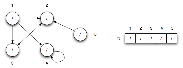
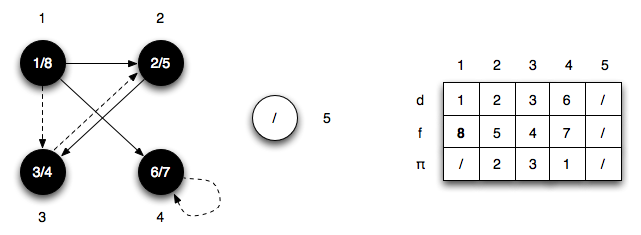
Consider the five node (directed) graph

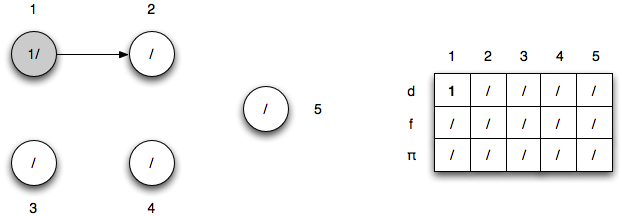
If we start at vertex 1 (and follow vertices in increasing numerical order), then

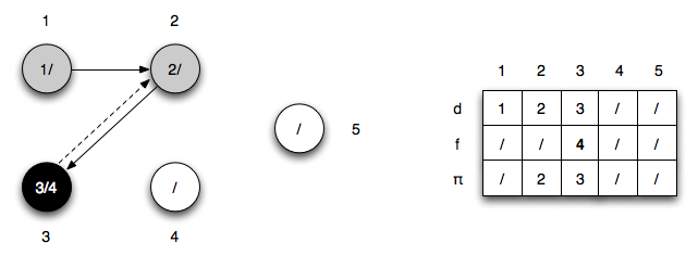
Timestep 1: u₁.d = 1 and we follow edge (u₁,u₂)

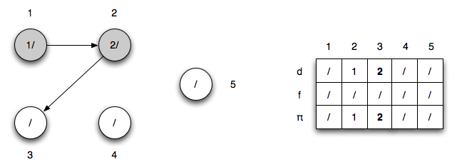
Timestep 2: u₂.d = 2 and we follow edge (u₂,u₃)

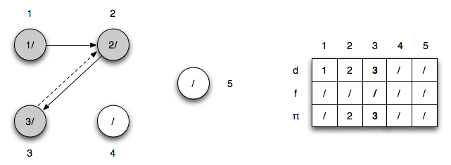
Timestep 3: u₃.d = 3 (note edge (u₃,u₂) is a back edge)

Timestep 4: there are no other edges to follow so u₃.f = 4

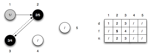
Timestep 5: there are no other edges to follow so u₂.f = 5

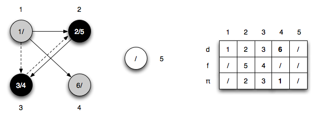
Timestep 6: follow edge (u₁,u₄) (note that edge (u₁,u₃) is a forward edge) so u₄.d = 6

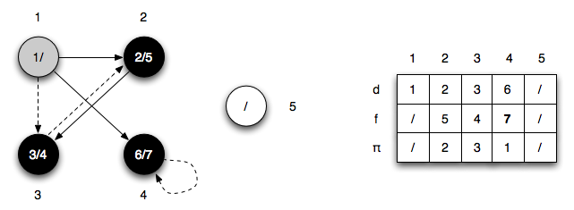
Timestep 7: there are no other edges to follow (note that edge (u₄,u₄) is a back edge) so u₄.f = 7

Timestep 8: there are no other edges to follow so u₁.f = 8

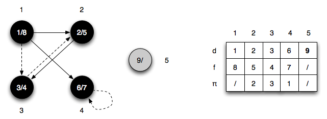
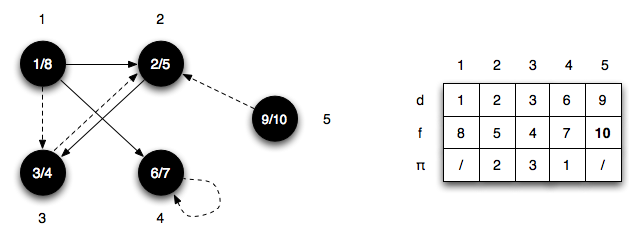
Timestep 9: there are no other edges to follow so begin a new tree at u₅.d = 9

Timestep 10: there are no other edges to follow (note that edge (u₅,u₂) is a cross edge) so u₅.f = 10

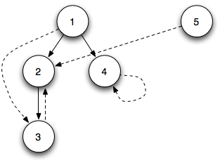
At this point there are no other white vertices so DFS terminates. The final depth-first trees are