CS 370: Lab 6: 3D Models, Perspective Projection, and Cameras

Orthographic projection is frequently used for third-person views (often static) where the objects are manipulated through transformations. However, when we create more realistic first-person views, we will use perspective projection where objects that are closer appear larger. Furthermore, particularly with perspective projection, where the viewer is, i.e. the camera location, will play an important role since the viewing volume will be defined relative to the camera’s position and orientation. Fortunately, OpenGL allows us to define the objects in world coordinates and then simply place the camera at the desired location with a specified projection without worrying about all the underlying transformations (since by duality it does not matter whether the camera is fixed and the objects move or the objects are fixed and the camera moves).

We can think of the process of projection as taking a “picture” of the world from a particular camera location. The particular camera model we will use is the simplified pinhole camera where the aperature is a single pinhole. Light rays are drawn from every point in the world, through the pinhole, and onto the projection plane (i.e. film). This particular method clearly will have the closest objects along each ray being the ones appearing in the final scene.

Since this model produces inverted images, we will assume that the projection plane is loacated an equal distance in front of the camera such that our images are right-side up.

We also will start rendering scenes with multiple objects. Rather than having to manually create geometry, especially for complicated objects, we will take advantage of models created with 3D modeling software, such as 3DS Max or Blender, and use a model loader to import the geometry into our applications and store each object in its own buffers for rendering.

Getting Started

Download CS370_Lab06.zip, saving it into the CS370-Fall2022 directory.

Double-click on CS370_Lab06.zip and extract the contents of the archive into a subdirectory called CS370_Lab06

Open CLion, select CS370-Fall2022 from the main screen (you may need to close any open projects), and open the CMakeLists.txt file in this directory (not the one in the CS370_Lab06 subdirectory). Uncomment the line

	add_subdirectory("CS370_Lab06" "CS370_Lab06/bin")

Finally, select Reload changes which should build the project and add it to the dropdown menu at the top of the IDE window.

Solution

Download CS370_Lab06_Solution.zip, saving it into the CS370-Fall2022 directory.

Double-click on CS370_Lab06_Solution.zip and extract the contents of the archive into a subdirectory called CS370_Lab06_Solution

	add_subdirectory("CS370_Lab06_Solution" "CS370_Lab06_Solution/bin")

Finally, select Reload changes which should build the project and add it to the dropdown menu at the top of the IDE window.

Model Loader

Since OpenGL does not provide support for loading models, we will use functions from the included utility library objloader.cpp. This loader works with files saved in the .obj format. Note: This loader does not support all the possible features that can be represented in an .obj file, but will load vertices, normals, and texture coordinates for the model (we will use normals and texture coordinates later in the course). While learning how to create complex models using modeling software will not be covered in this course, in a subsequent lab we will briefly learn how to generate some simple geometric shape models using Blender. The function to load an .obj model is

void loadOBJ(const char *path, vector<vec4> &out_vertices, vector<vec2> &out_uvs, vector<vec3> &out_normals);

where path is the path to the .obj model file, out_vertices is a reference to a vector<vec4> (similar to an ArrayList in Java) to return the vertices, out_uvs is a reference to a vector<vec2> to return the texture coordinates (which we will use when we discuss texture mapping), and out_normals is a reference to a vector<vec3> to return the face normals (which we will use when we discuss lighting). Once we have loaded the information from the model into the return vectors, we can place these into our buffers for subsequent rendering. Since color information is not stored in the .obj file, we will create additional color buffers and add a color per vertex for each object using the utility routine

void build_solid_color_buffer(GLuint numVertices, vec4 color, GLuint buffer);

where numVertices is the number of vertices (i.e. colors) for the object we are building a color buffer for, color is the color we want to use, and buffer is the index into the ColorBuffers array we wish to create.

The models can then be rendered using a simple utility function which will bind the buffers passed as parameters and draw the geometry using GL_TRIANGLES

void draw_col_obj(GLuint obj, GLuint color);

where obj is the VAO_IDs for the object we wish to draw and color is the Color_Buffer_IDs* of the color we wish to use (which must have the same number of colors as the object has vertices).

Tasks

NOTE: The global vector objFiles contains the filenames for the .obj files which are stored in the models subdirectory for the project.

Add code to load_object() to load the model indexed by obj. Hint: Use the objFiles vector (whose elements can be accessed using [] like arrays), and pass references to the vertices, uvCoords, and normals vectors (you do not need & since vectors are objects). Assign the obj index of the numVertices[] array to the size of the vertices vector (using the .size() method). Subsequent code is provided to create and load the vertex data into the attribute buffers for the object.
Add code to build_geometry() to load the Cube model. Hint: Use the Cube constant with the load_object function.
Add code to build_geometry() to load the Sphere model. Hint: Use the Sphere constant with the load_object function.
Add code to build_geometry() to build a red color buffer for the Cube model. Hint: Use the Cube element of the numVertices array, a vec4(1.0f, 0.0f, 0.0f, 1.0f) color, and the CubeRed buffer id with the build__solid_color_buffer() function.
Add code to build_geometry() to build a yellow color buffer for the Sphere model. Hint: Use the Sphere element of the numVertices array, a vec4(1.0f, 1.0f, 0.0f, 1.0f) color, and the SphereYellow buffer id with the build__solid_color_buffer() function.
Add code to render_scene() to draw the cube object using the draw_color_obj() function. Hint: Use the Cube and CubeRed constants.
Add code to render_scene() to draw the sphere object using the draw_color_obj() function. Hint: Use the Sphere and SphereYellow constants.

Even though we should be rendering two objects, they will not appear as we have not set an appropriate viewing volume and positioned the camera such that they are visible.

Perspective Projection

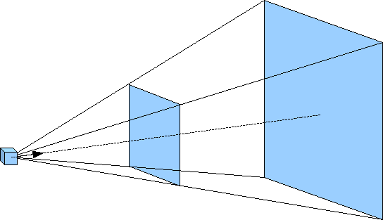
Unlike orthographic projection where parallel lines remain parallel and the size of an object is independent of its location relative to the camera, perspective projection is more akin to actual scenes. For example, two parallel railroad tracks appear to converge to a point in the distance and as objects move away from the observer, i.e. the camera, they get smaller in size. For this projection mode, rather than the viewing volume being a parallelapiped, it has a shape known as a frustum. This frustum can be visualized as a pyramid with its point at the camera but starting a small distance in front of the camera (known as the near clipping plane) and extending a further distance outward (known as the far clipping plane) as shown below.

For a perspective projection, we will set the projection matrix by creating a frustum viewing volume with our desired extents (of the near clipping plane) using

mat4 frustum(float left, float right, float bottom, float top, float near, float far);

where again left and right are the x extents of the near clipping plane, bottom and top are the y extents of the near clipping plane, and near and far are the z extents in world coordinate units of the near and far clipping planes respectively FROM THE POSITION OF THE CAMERA in a direction along the camera’s axis. The default position for the camera is the world origin looking back down the z axis. However since the camera now is within the scene, near must be positive and far > near (be careful not to make near too small).

Note: The larger and closer the near clipping plane is to the camera, the more the projection will cause distortion. A good rule of thumb to begin with is to set the x and y extents and the near clippling plane distance to the same values until the objects are in the scene, and then make adjustments to achieve the desired effect.

Tasks

Add code to display() to set proj_matrix to an anisotropic frustum projection with nominal extents [-1.0,1.0] for x and y, the near clipping plane 1 unit in front of the camera, and the far clipping plane 8 (or more) units in front of the camera.

While we have now set a reasonable viewing volume, the default camera is currently inside the cube (at the origin) with a near clipping plane beyond the back of the cube (and we are also culling back faces). See what happens if you disable back face culling and adjusting the near clipping plane distance.

Camera Position

The default camera position is at the origin pointed in the -z direction, i.e. you are the center of the universe. We can, however, create a matrix to change this position and orientation using

mat4 lookat(vec3 eye, vec3 center, vec3 up);

where eye are the world coordinates of the camera, center are the world coordinates where the camera is pointing, and up define a vector indicating which direction is up for the camera (since otherwise the camera could have any orientation about the axis defined by eye and center).

Essentially, placing a camera in the scene transforms all objects in the scene from the world coordinate system to the camera coordinate system, i.e. creates a global transformation. Thus, typically it will be created in the the display() function and later we will see that it gets multiplied in the shader prior to the modelview transformations. Note: If we wish to have some objects remain stationary with respect to the camera, e.g. a heads up display, we can either skip multiplying the camera transformation or set it (temporarily) to the identity matrix.

Tasks

Add code to display() to set camera_matrix to position the camera at location eye pointed at location center oriented using up.

Now you should be able to see the objects rendered with a perspective projection.

Spherical Coordinates

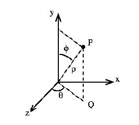
Often times when we wish to move the camera through a scene, simply adjusting the (x,y,z) components of the eye vector (with a corresponding adjustment of center) in Cartesian coordinates produces awkward behaviors. Instead, especially in a third person view, it is more natural if the camera is moved in spherical coordinates which consist of an azimuth angle (rotation about the y axis), an elevation angle (rotation down from the y axis), and a radius (distance from the origin), see the diagram below

With this coordinate system, the camera appears to move around a sphere such that it rotates around the scene (azimuth), “up/down” in the scene (elevation), and “towards/away from” the center of the scene (radius). However, since lookat strictly uses Cartesian coordinates (i.e. (x,y,z)) the conversion from spherical to Cartesian coordinates is given by

I have included code in the lab to initialize eye in main() and update it in key_callback() to revolve the camera around the scene by adjusting the azimuth and elevation angles using WASD and zooming in/out by adjusting the radius using ZX, and then recomputing the eye vector.

Compiling and running the program

You should be able to build and run the program by selecting frustumScene from the dropdown menu and clicking the small green arrow towards the right of the top toolbar.

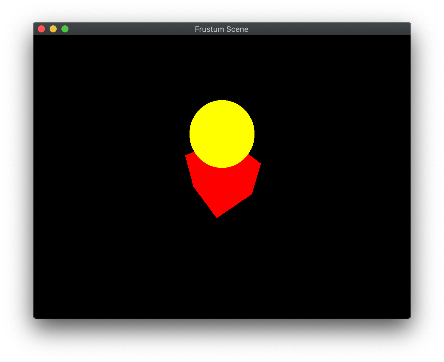
At this point you should see a red cube with a yellow sphere on top of it and be able to move the camera around the objects.

To quit the program simply close the window.

Congratulations, you have now created a perspective scene and added a camera.

Next we will discuss more about the programmable shaders and how they are used to render our geometry.